Introduction
Gaia relies on the proven principles of ESA’s Hipparcos mission to help solve one of the most difficult yet deeply fundamental challenges in modern astronomy: the creation of an extraordinarily precise three-dimensional map of about one billion stars throughout our Galaxy and beyond.
Gaia Mission – Gaia – Cosmos
On this exercise usage of the Gaia data will be demonstrated by two approaches. Both utilize TAP protocol to access the data, but the first approach will use dedicated software – TOPCAT, and the second approach will use python software library to access the data programmatically.
Lecture slides
Files for this exercise
- All files are available in the git repository stored in the faculty’s Gitlab server.
- The address of the project is the following:
https://git.kpi.fei.tuke.sk/svd/gaia-lab-base-svd - Repository for lecturers:
https://git.kpi.fei.tuke.sk/mv120fd/gaia-lab-svd-for-teachers
Setup of the environment
- Setup of the python environment
- The python and necessary libraries can be installed locally, or the examined jupyter notebooks can be run in cloud-based solutions such as Google colaboratory.
- Python 3.X installation
- Follow the installation steps for your specific platform. For instance, nice installation guide is available at https://realpython.com/installing-python/.
- Environment setup:
- Virtual environments (venv, conda) are recommended for the local installation.
- Virtual environment can be set-up by the following command:
python3 -m virtualenv -p python3 venv
# activation
. venv/bin/activate
- Virtual environment can be set-up by the following command:
- Required non-standard libraries are listed in requirements.txt file
- With pip package installer, all required packages can be installed via:
pip install -r requirements.txt - With conda package installer, all required packages can be installed via:
conda env create -f environment.yml - To use files in Google Drive (such as requirements.txt), the Google Drive directories can be mounted in a notebook using google.colab.drive library (see the example notebook). Shell commands can be executed from a jupyter notebook by putting an exclamation point as the first letter of a line (example of shell commands in IPython).
- Virtual environments (venv, conda) are recommended for the local installation.
- TOPCAT installation
- The appropriate executable/jar can be downloaded from the project’s website: http://www.star.bris.ac.uk/~mbt/topcat/#install
Summary of the activities
Astroquery Gaia TAP example (Jupyter)
Astroquery Gaia TAP example.ipynb- The notebook illustrates synchronous TAP query using astroquery.gaia module, some possibilities to show data of astropy.Table, and finally visualization of the data using scatter plot without any modifications.
- The rendering of the sky does not adhere to the conventions used in astronomy. See the next notebook which examines this topic.
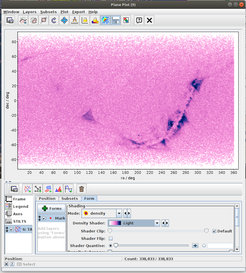
Skymap coordinates plotting (Jupyter)
Skymap plots in matplotlib.ipynb- This notebook demonstrates plotting of a subset of Gaia data in galactic coordinates using Matplotlib library. Although it is easy to use, Matplotlib is not ideal for plotting sky map coordinates, and additional fixes are required to plot the data in a more conventional way.
- The data are loaded from a file created by the previous notebook (only a sample of 10000 random entries).
Plotting Number of sources per subarea of the sky using ADQL (Jupyter)
Number of sources per subarea of the sky using ADQL.ipynb- Task #1: Finish the ADQL query
- Bin galactic longitude and galactic latitude into bins of size 5 degrees.
- Use division by the bin size and round the result (for instance by FLOOR function)
- Group subquery results by longitude and latitude bin.
- Don’t forget to rescale-back the values after division.
- Returned longitude and latitude values as bin center values.
- Required columns are the following: source_id_count, l_bin_center, b_bin_center
- Applied plotting approach, might be puzzling. It transforms the table data into a grid of pixels almost in one line. However, it requires identical number longitude bins of rows of each latitude bin.
- The notebook shows another functioning method for rendering mollweide projection-based histogram.
- Task #2: Make a copy of this notebook and instead of the number of sources plot total luminosity at a particular location.
Plotting Number of sources per healpix pixel using ADQL (Jupyter)
HEALPix examples.ipynb- Task #1: Extract HEALPix pixel identifier from gaia source ID using an appropriate equation. Calculation of the HEALPix index can be found in the Datamodel documentation (see: Nigel Hambly et al. Gaia DR2 Documentation, Datamodel description: gaia_source. https://gea.esac.esa.int/archive/documentation/GDR2/Gaia_archive/chap_datamodel/sec_dm_main_tables/ssec_dm_gaia_source.html).
- Task #2: Finish ADQL query to group sources by their healpix pixel at order 5. For available HEALPix-specific ADQL functions see Gaia Archive Help (https://gea.esac.esa.int/archive-help/adql/index.html).
- Task #3: Finish implementation of the code for plotting the whole sky map in RGB.
- R – mean red photometer flux, B – mean blue photometer flux, G – mean G-band photometer flux.
- The indices in the table (column ipix) are in order/level of 8.
- Use Mollweide projection, use coord argument to translate celestial (equatorial) coordinates. (see: https://healpy.readthedocs.io/en/latest/generated/healpy.visufunc.mollview.html)
Estimated distance of a source (Jupyter)
Estimated distance of a source.ipynb- The notebook illustrates usage of the external table in the Gaia archive, which contains precomputed distances to many sources in the gaiadr2.gaia_data table.
- The table is a result of work done by C.A.L. Bailer-Jones et al. in paper titled “Estimating distances from parallaxes IV: Distances to 1.33 billion stars in Gaia Data Release 2” (see: https://arxiv.org/abs/1804.10121).
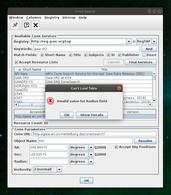
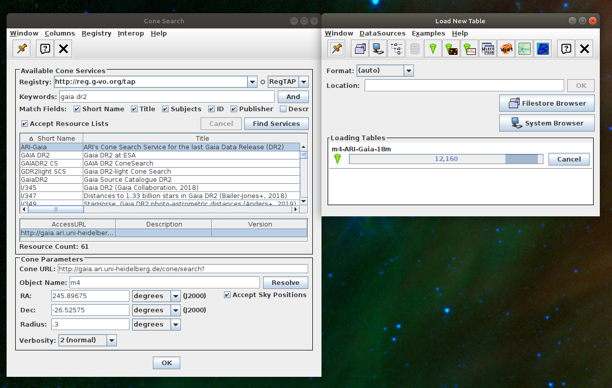
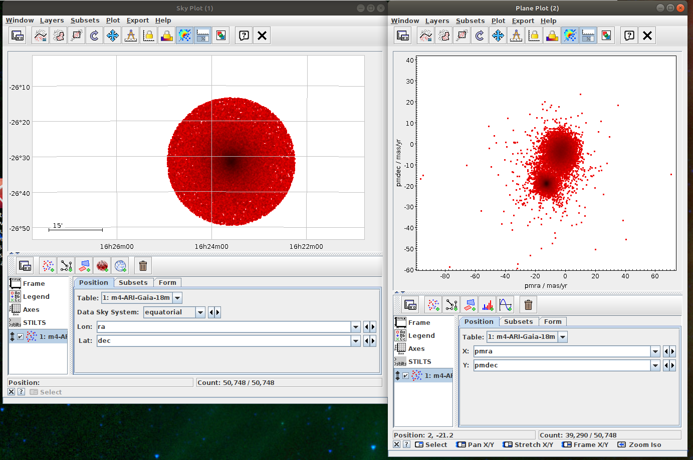
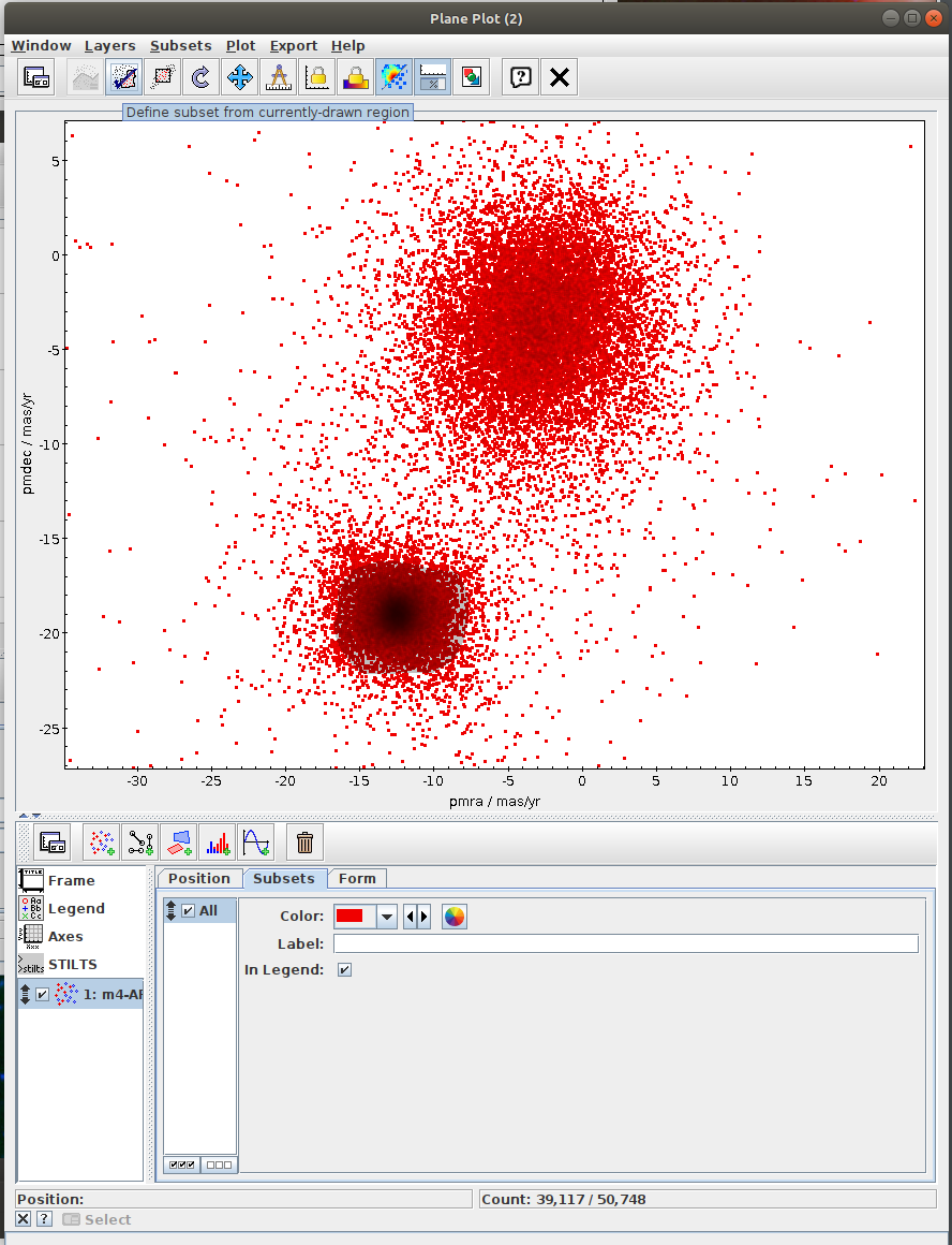
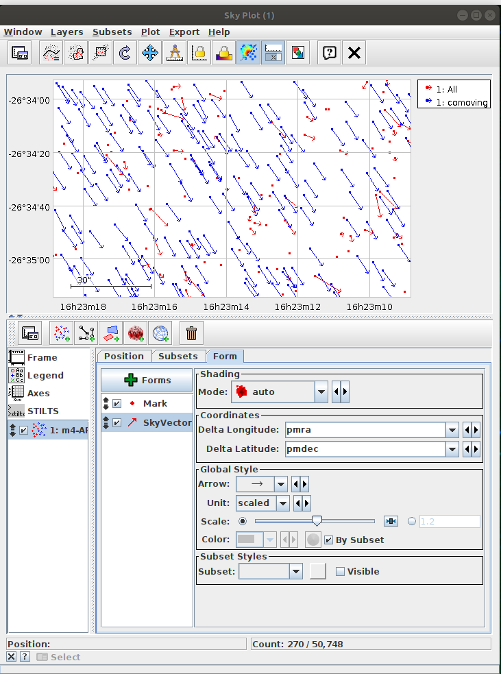
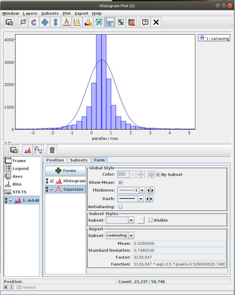
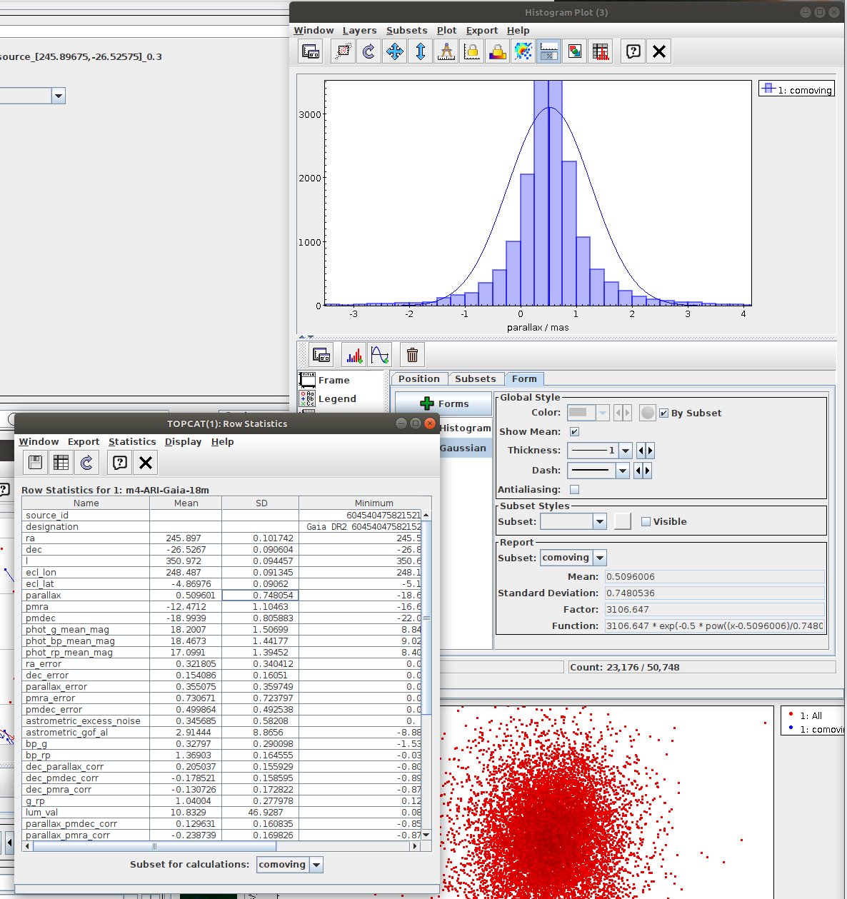
Messier 4 in proper motion space (TOPCAT)
- Task #1 in TOPCAT tutorial by Mark Taylor

Messier 4 in proper motion space (Jupyter)
Cluster identification n1 Messier 4 in proper motion space.ipynb- This notebook is python reproduction of a tutorial by Mark Taylor. It is the first tutorial in the document linked below. The tutorial focuses on identification of a star cluster in the proper motion space.
- Task #1: Implementation of clustering (DBSCAN)
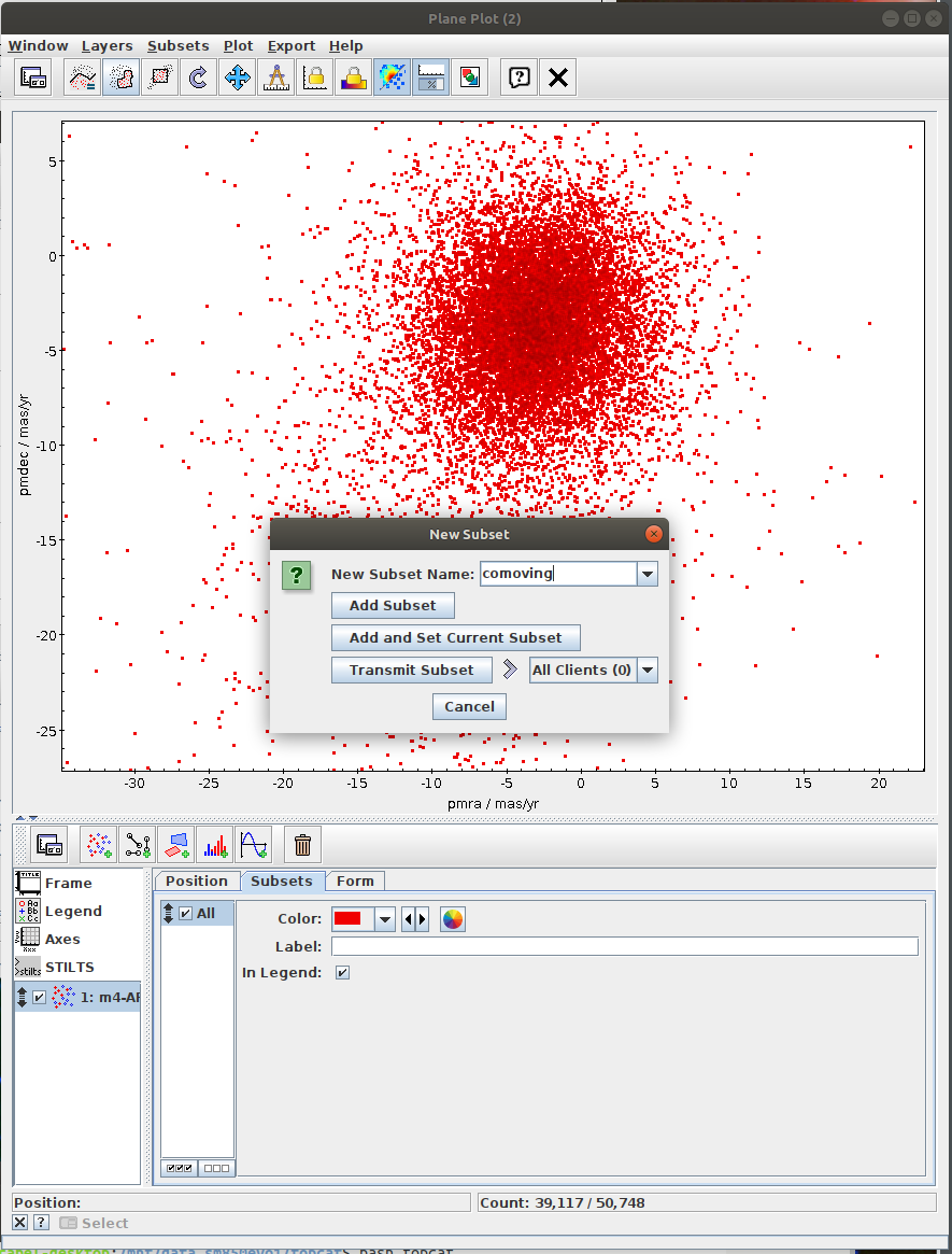
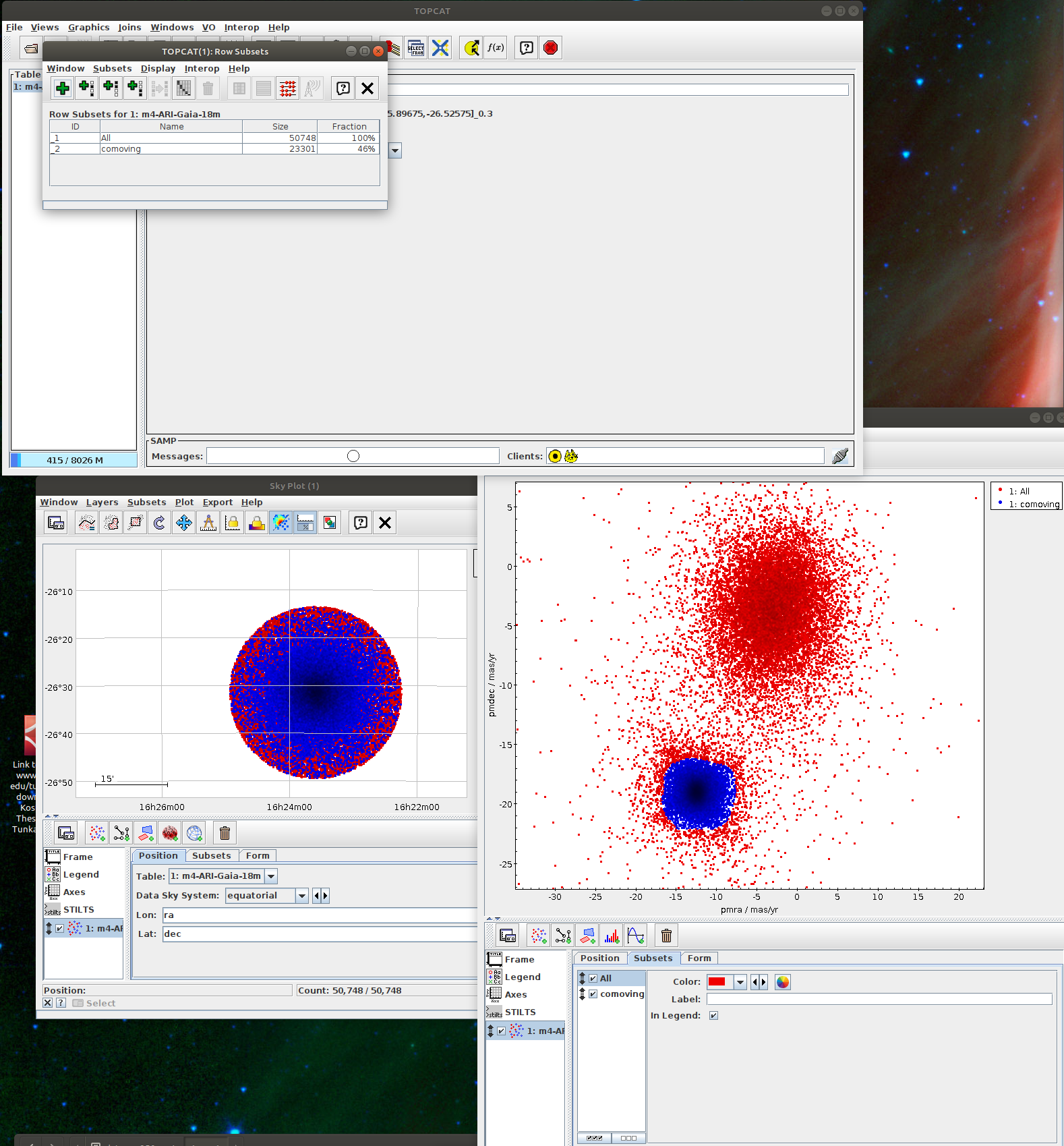
Aim of the task is to separate the clusters in the proper motion space. The recommended method here is to use clustering instead of selecting sources in a manually specified region. - Task #2: Select the “comoving” cluster out of the identified clusters
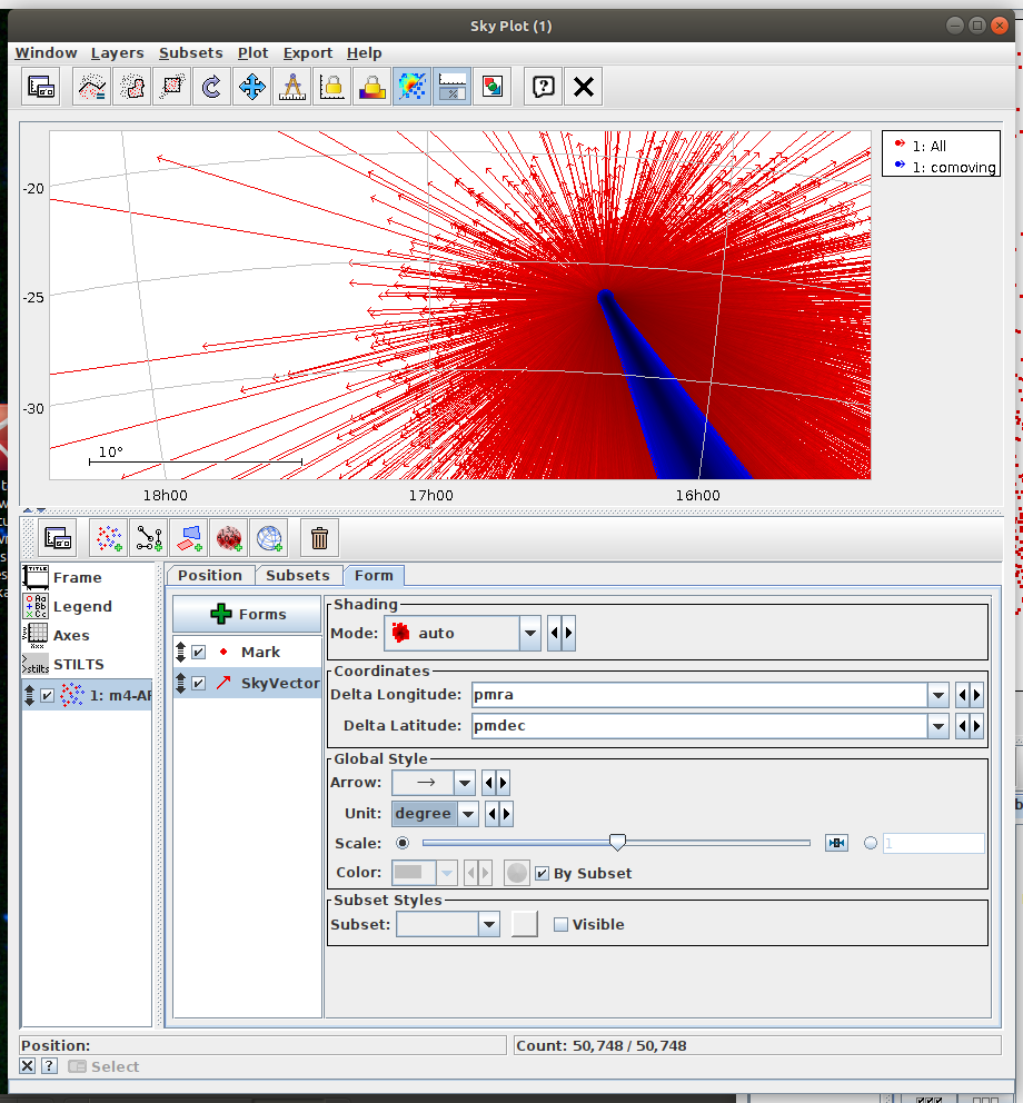
Assign the “commoving” cluster’s label to the variable comoving_cluster_label - Task #3: Visualize proper monition using Matplotlib.Axes.arrow
- Draw arrows marking the proper motion vectors.
- Make the celestial coordinates start points of the arrows.
- Scale proper motion values to fit into the image.
- For drawing the arrows, you can use matplotlib.axes.Axes.arrow. Recommended options: width=0.00005, linewidth=0, head_width=0.0005
- Compare the resulting image with the TOPCAT result.
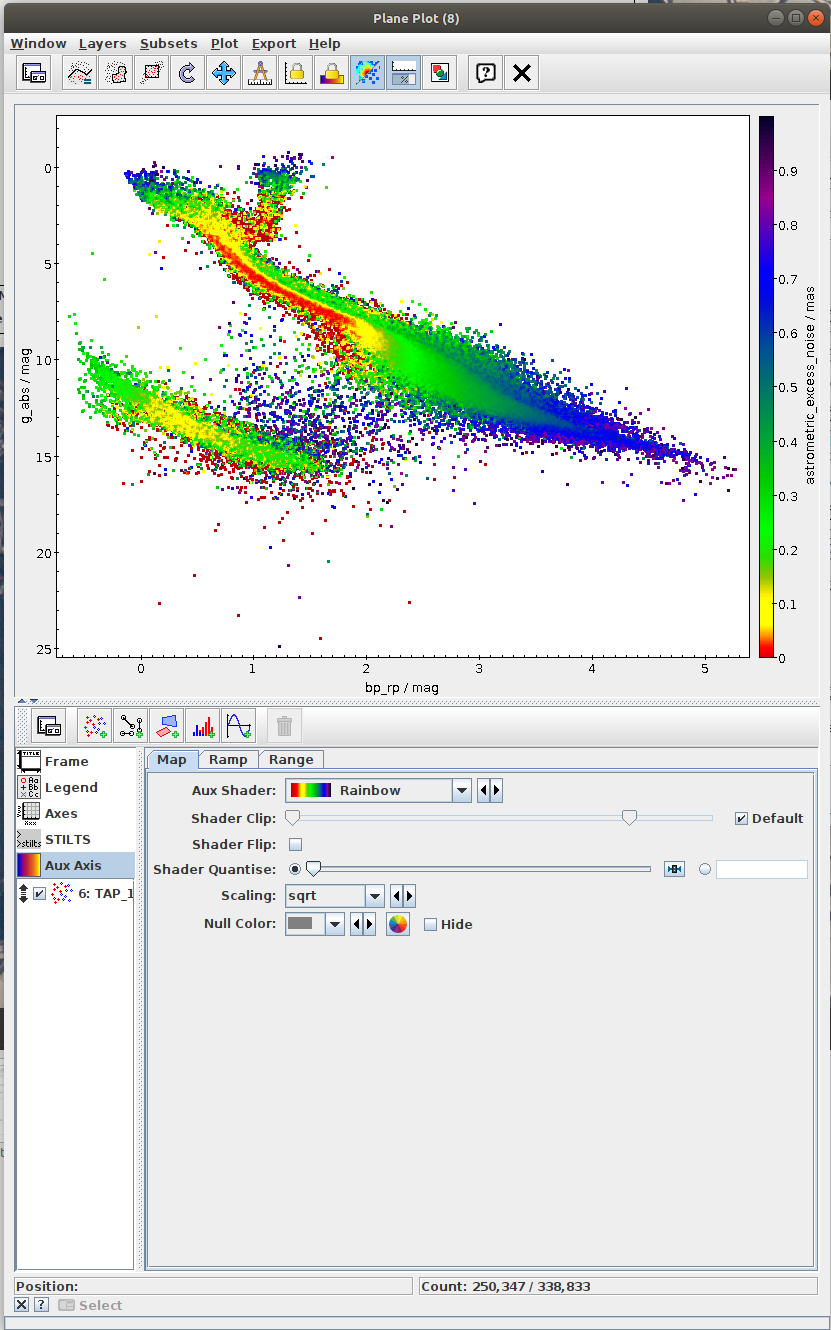
Hertzsprung-Russell diagram for a subset of sources (TOPCAT)
- Task #4 in TOPCAT tutorial by Mark Taylor
- Very nice visualization explaining the Herzsprung-Russell Diagram (HRD) is available at https://sci.esa.int/gaia-stellar-family-portrait/. In this diagram the stars are found in different regions depending on their masses, ages, and stages in the stellar life cycle.

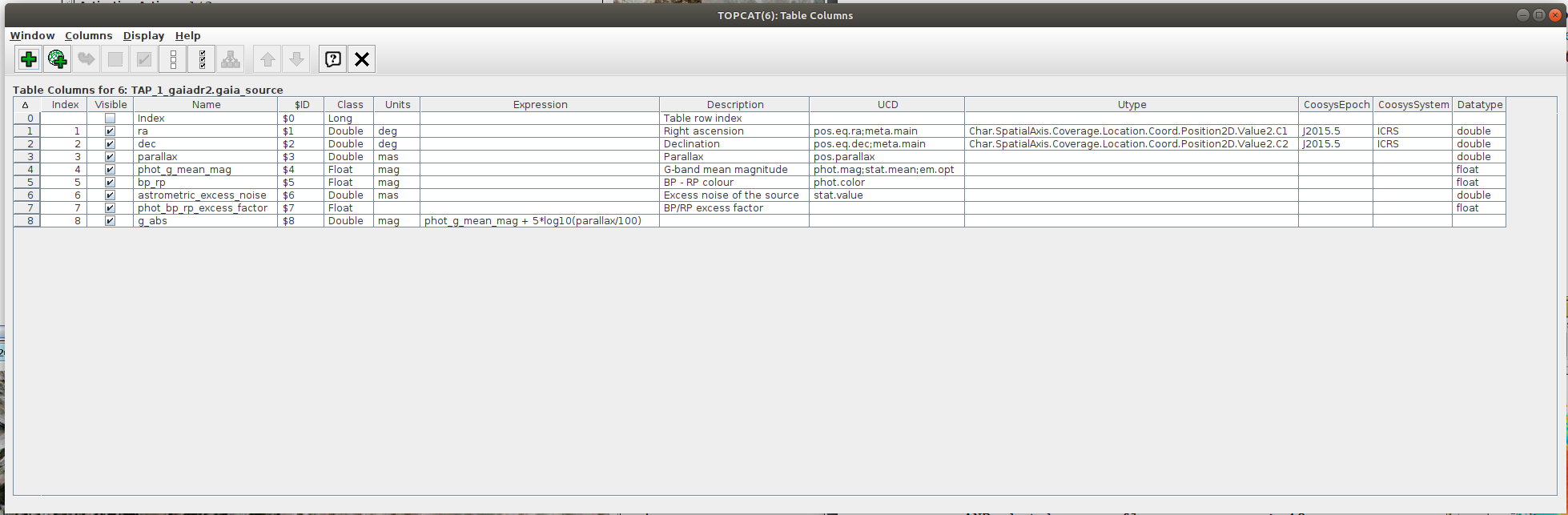

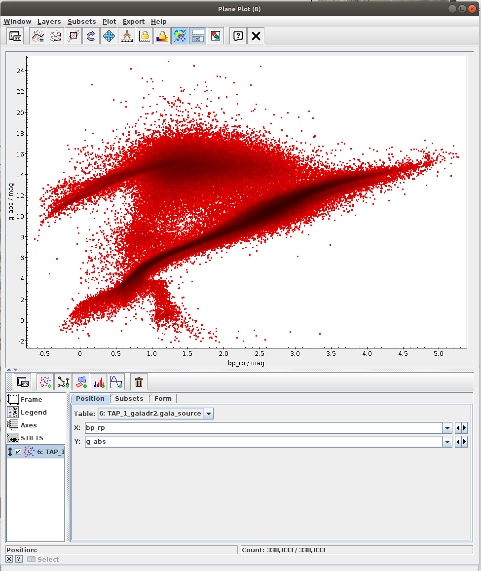
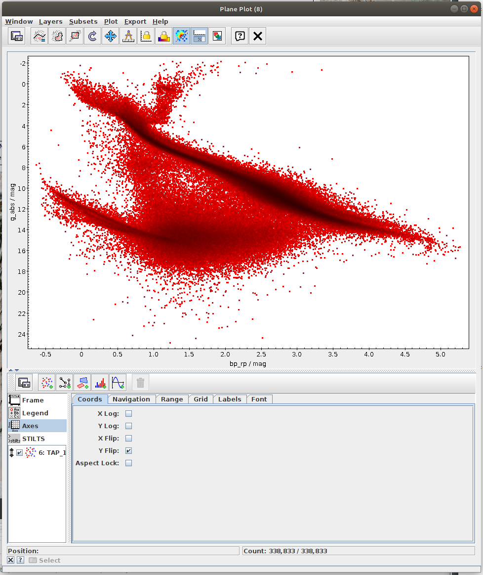
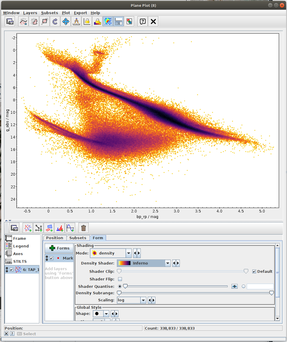

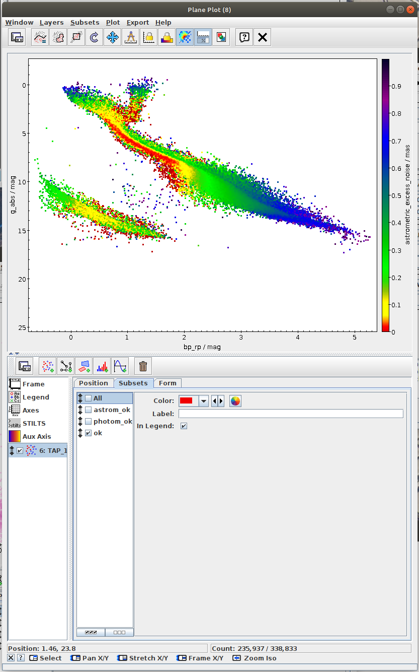

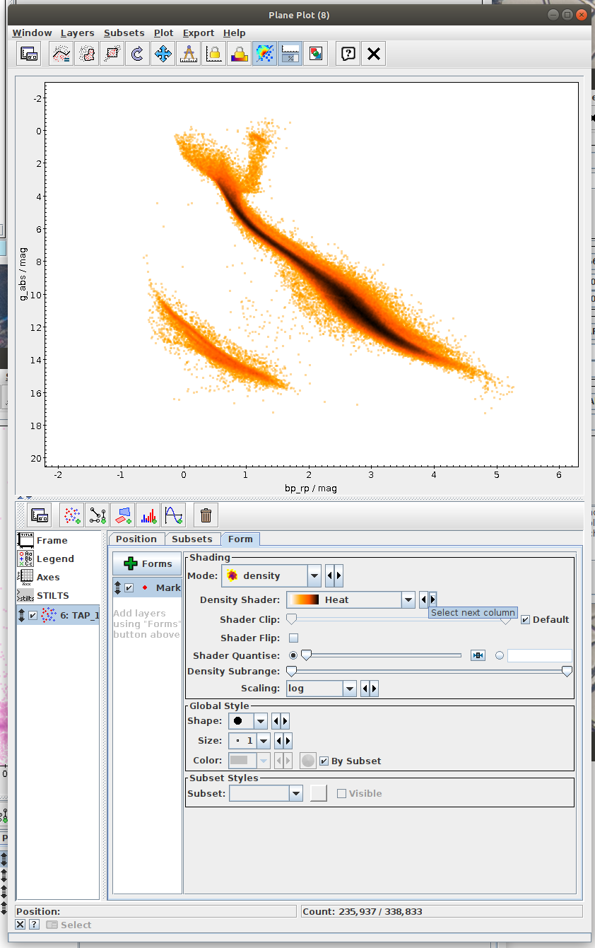
Hertzsprung-Russell diagram for a subset of sources (Jupyter)
Local Herzsprung-Russell Diagram.ipynb- This notebook is python reproduction of a tutorial by Mark Taylor. It is the fourth tutorial in the document linked below. The tutorial focuses on plotting Local Herzsprung-Russell Diagram from Gaia data.
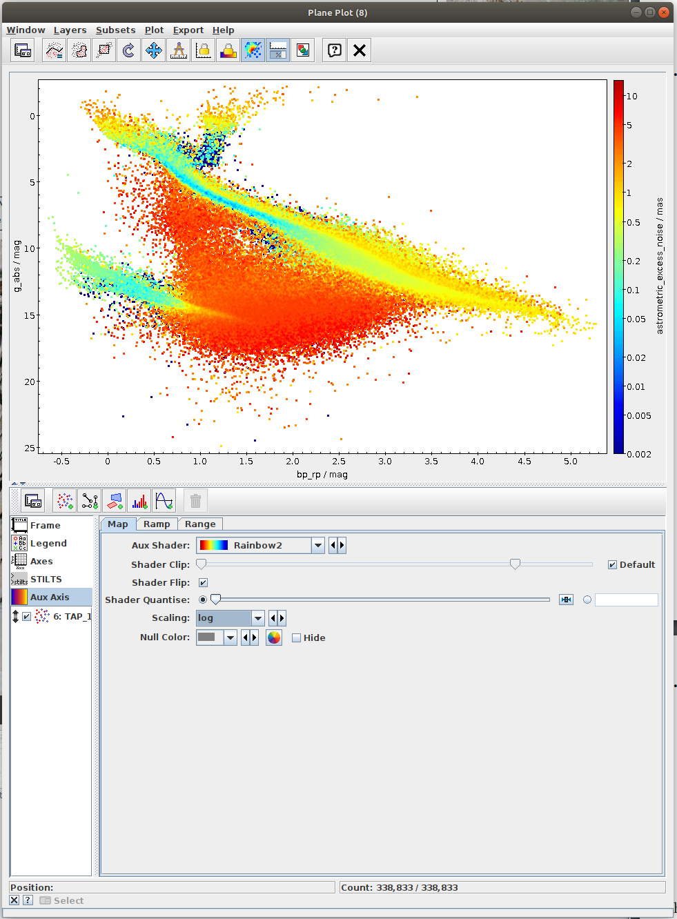
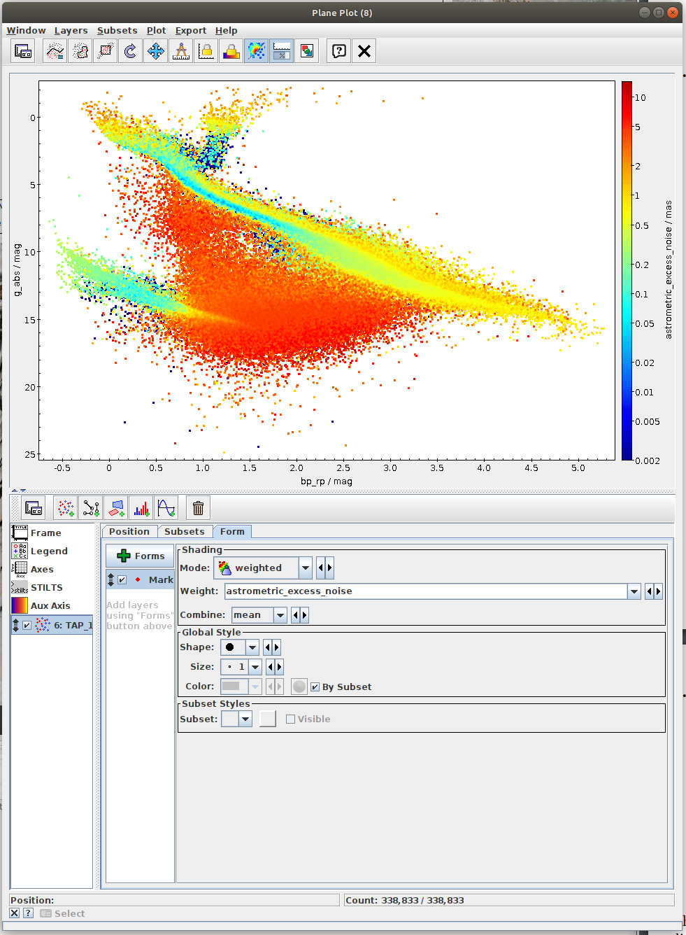
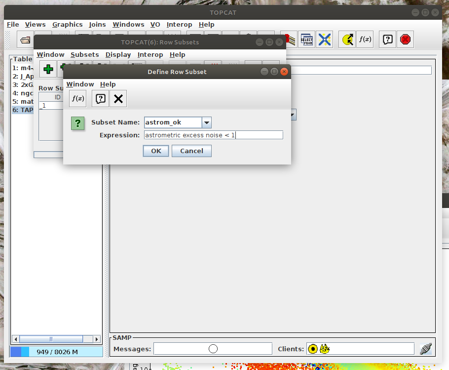
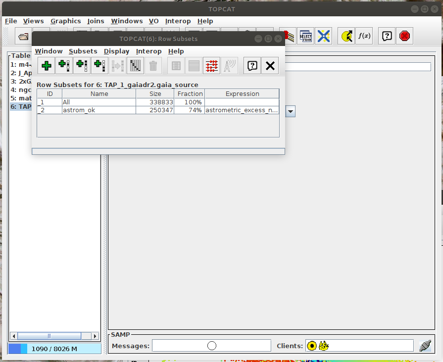
- Task #1: Calculate mean values of astrometric_excess_noise per each bin.
One possibility is to use scipy.stats.binned_statistic_2d. In the case of this function, it might be necessary to resolve NaN values. This can be done by np.nan_to_num. - Task #2: Apply a cut on the astrometric excess noise and create a filtered subset.
- Apply a cut to select only sources with astrometric_excess_noise under 1
- Calculate 2D binned statistic (for instance using scipy.stats.binned_statistic_2d
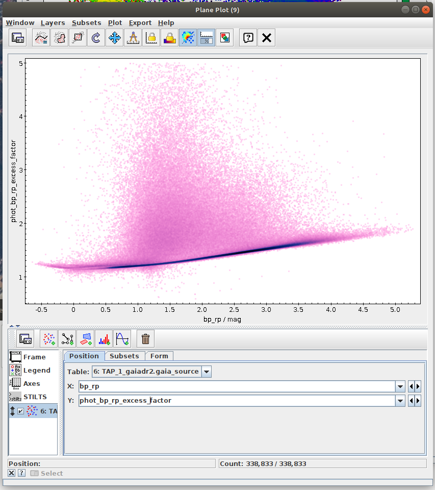
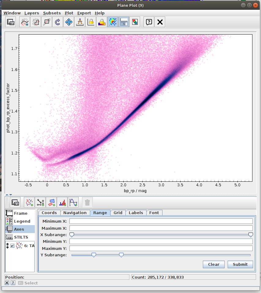
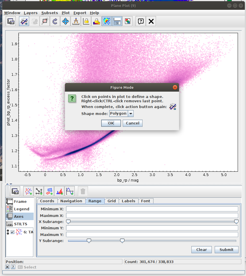
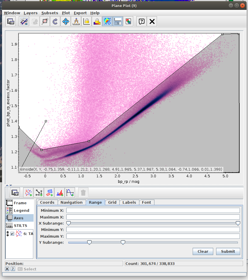
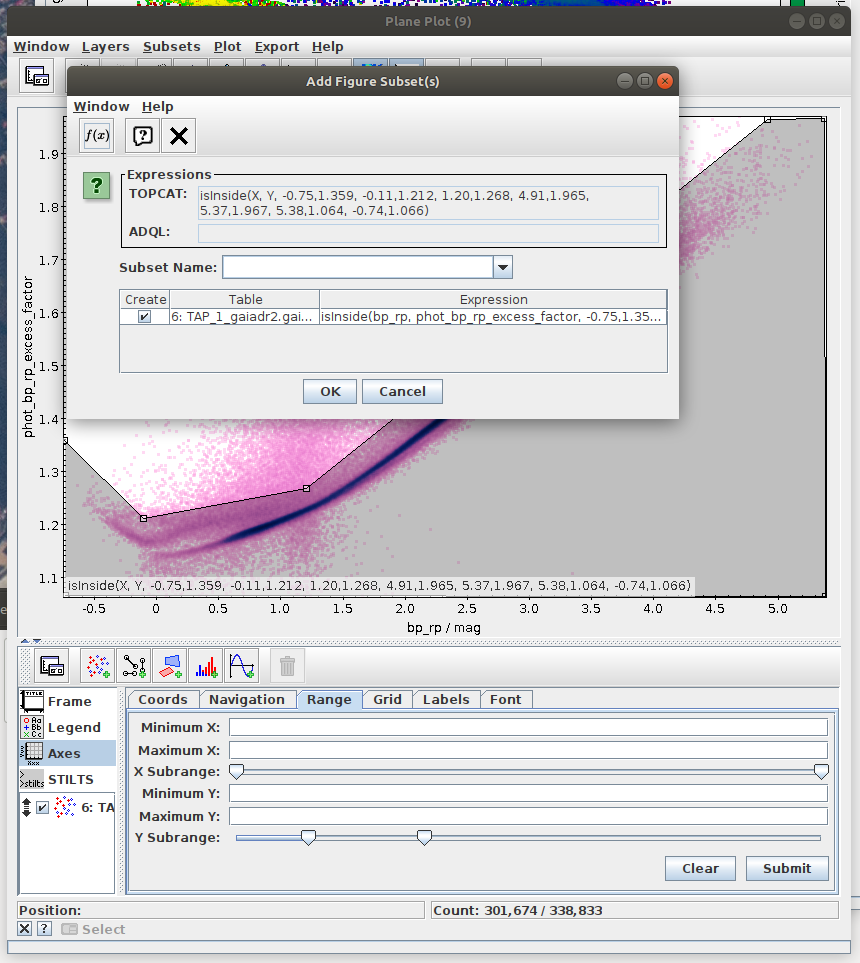
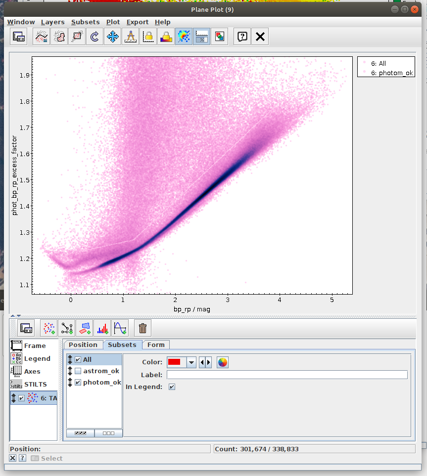
- Task #3: Apply a cut based on the predefined polygon in the space defined by BP-RP colour and BP/RP excess factor.
Create a mask of sources which are contained inside the predefined polygon.
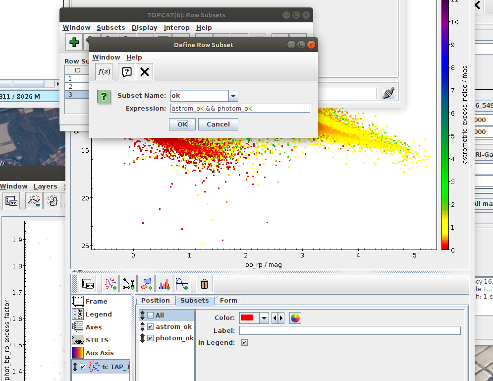
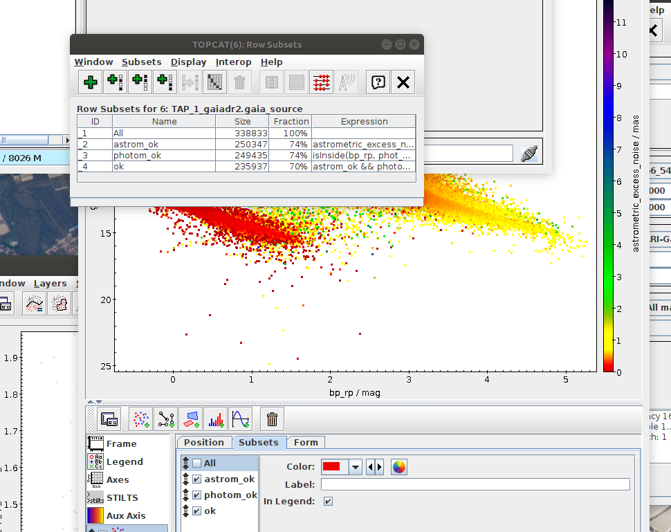
Possible inspiration: - Task #4: Apply both photometric and astrometric-cut masks on the original data from the archive.
- Create a subset of data satisfying both photometric and astrometric cuts (OK subset). Create a combined mask of the photometric and astrometric mask and use it to filter the data. Save a reference to the filtered dataset into variable gaia_data_ok.
- Create a 2D array of the binned statistic for the OK subset. You can copy and modify code from the task #2. Save a reference to the filtered dataset into variable bin_means_ok.
Hertzsprung-Russell diagram in single ADQL (Jupyter)
Herzsprung-Russell Diagram from ADQL Mora et al.ipynb- The notebook shows an example of creation of the similar histogram as the previous example, but here summation and more detailed filtration is done in the ADQL query, which also includes cross-match with an external catalogue available through the Gaia archive.
ADQL query is taken from a presentation by A. Mora et al. at IAU Symposium 330. Nice, France. The slide are available here: https://iaus330.sciencesconf.org/data/pages/Mora.pdf