Similarly to cosmic ray physics, the topic is closely related to the activities of IEP. The lesson is planned to work with data from the Parker Solar Probe mission. The students should be introduced to methods of acquiring and reading the mission’s data. They should be able to visualize and understand them on a basic level. The discussed topics will include the dependence of solar wind from helioaltitude, dynamic pressure, and others.
Lecture slides
Lab activities
- All files are available in the git repository stored on the faculty’s Gitlab server.
- The address of the project is the following:
https://git.kpi.fei.tuke.sk/svd/lab-cosmic-rays
The activity named “Reading Cosmic Ray Spectra Files and Fitting Spectra to a Model” includes the following:
- Implementation of equations describing a model (force field approximation) in a program.
- Loading data from two cosmic ray spectra archives.
- Fitting the model to measured spectra.
The Jupyter notebook partially reproduces plots presented in an article by Ilya G. Usoskin and others.
Usoskin, I. G., A. Gil, G. A. Kovaltsov, A. L. Mishev, and V. V. Mikhailov, (2017), Heliospheric modulation of cosmic rays during the neutron monitor era: Calibration using PAMELA data for 2006–2010, J. Geophys. Res. Space Physics, 122, 3875–3887, doi:10.1002/2016JA023819
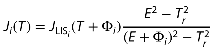
TASK #1: Implement the equation for the Force Field Approximation into the code
- Implement it inside the function calc_J(T, Phi, T_r).
- Use the function `calc_J_LIS` to calculate the value of JLIS. Don’t forget to pass T + Φi as the parameter value of the function.
TASK #2: Select only entries associated to the paper identified by ads url equal 2013ApJ…765…91A
- Store a reference to the resulting dataset in variable pamela_only_H_etot_2006_df
- You can use your preferred method out of several possibilities in Pandas
TASK #3: Filter-out only entries where sub_exp is equal to PAMELA(2006/08-2006/09)
- Store a reference to the resulting dataset in variable pamela_only_H_etot_2006_08_09_df
- You can use your preferred method out of several possibilities in Pandas
TASK #4: Visualize the fitted model alongside the measured PAMELA data
- Run the model function with the fitted value of Φ.
- Visualize both weighted and unweighted variant
- Provide appropriate labels which will include the fitted value of Φ parameter
TASK #5: Perform a fit of the model only on the data specified by the range of energie in variable energy_range
- Based on the code above, first, perform the fit (weighted or non-wighted)
- Visualize results and compare the following:
- the actual data,
- the model fitted to whole spectrum,
- the model fitted only to the values associated with the energies inside the range.
TASK #6: Go to the Cosmic ray database (https://tools.ssdc.asi.it/CosmicRays/) and download all PAMELA spectra associated to paper ApJ 765 (2013) 91*
- Open the website: https://tools.ssdc.asi.it/CosmicRays/
- In the Search form specify the following parameter values:
- Particle: p (which stands for proton)
- Plot: Flux vs Kinetic Energy
- Experiments: PAMELA
- Wait for the search to complete
- Select spectra associated to the paper ApJ 765 (2013) 91.
- Click on Plot Selected
- Observe the image and click on Download button. Keep the checkboxes for all available formats checked.
- Extract the downloaded data into directory data/pamela/ssdc_cosmicrays_2021-03-04/
TASK #7: Read the file form the COSMIC RAY Database (https://tools.ssdc.asi.it/CosmicRays/)
- Based on the printout above, use appropriate parameter values of read the file using pandas.read_csv
- Think about specifying a correct separator, column names, comment character
- See:
TASK #8: Visualize the fitted model alongside the data form the SSDC’s Cosmic ray archive
- Base your implementation on the code used earlier
TASK #9: Calculate the missing mean value of the kinetic energy
- Use columns ‘kinetic_energy_min’,’kinetic_energy_max’
- Attempt to utilize DataFrame.mean function
- See:
TASK #10: Fit the model to the data loaded form the XML file
- Base your implementation on the code above, but keep in mind the different column names
TASK #11: Use Series.map function on filenames in the index data frame (ssdc_file_index_df)
- Use function fit_Phi_on_ssdc_cr
- See: