Earth observation is the gathering of information about planet Earth’s physical, chemical and biological systems via remote sensing technologies, usually involving satellites carrying imaging devices. Earth observation is used to monitor and assess the status of, and changes in, the natural and manmade environment.
Earth observation | EU Science Hub, CC BY 4.0
On this exercise usage of the Gaia data will be demonstrated by two approaches. Both utilize TAP protocol to access the data, but the first approach will use dedicated software – TOPCAT, and the second approach will use python software library to access the data programmatically.
- Lecture slides: Lecture 1, Lecture 2, Lecture 3
- Files for this lab
- Setup of the environment
- Summary of the lab activities
- Detailed description of lab activities
- Recommended reading
Lecture slides
Earth Observation – Copernicus I.
The lecture focuses on general description of the Copernicus programe and platforms for data access.
Earth Observation – Copernicus II.
The lecture focuses on description of basic concepts and data analysis methods.
Earth Observation – Copernicus III.
The lecture focuses on general description of data formats used in the field of Earth Observation and overviews software and libraries used in the analysis of Earth Observation data.
Files for this lab
- All files are available in the git repository stored in the faculty’s Gitlab server.
- Address of the project is the following:
- Repository for students:
https://git.kpi.fei.tuke.sk/svd/lab-earth-observation
- Repository for students:
- PIP environment specifications in the repository:
- requirements.txt
- requirements_OCEA01.txt
- Jupyter notebooks with tasks:
- OCEA01.ipynb
- NetCDF – C3S Fire Warning Indicator – multiple files.ipynb
- NetCDF – C3S Fire Warning Indicator – single file.ipynb
- NetCDF from Sentinel 3 OLCI.ipynb
- WMS s2cloudless.ipynb
- Per-pixel classification – 1. preparation of datasets – PART1.ipynb
- Per-pixel classification – 1. preparation of datasets – PART2.ipynb
- Per-pixel classification – 1. preparation of datasets – PART3.ipynb
- Per-pixel classification – 2. training.ipynb
- Per-pixel classification – 3. application.ipynb
- Demonstrative Jupyter notebooks:
- GRIB – C3S Essential climate variables.ipynb
- Affine example.ipynb
- Fiona example.ipynb
- Per-pixel classification – misc – cloud masks.ipynb
- Read shapefile in Geopandas.ipynb
- Script for Google Earth Engine:
- ndvi_ndwi_google_earth_engine.js
Datasets used in the lab
C3S Climate Data Store
- Fire danger indicators for Europe from 1970 to 2098 derived from climate projections
- Time aggregation: Seasonal indicators
- Product type: Multi-model mean case
- Variable: Seasonal fire weather index
- Experiment: RCP4.5
- Period: 2006-2010, 2011-2015, 2016-2020, 2021-2025, 2021-2040, 2026-2030, 2031-2035, 2036-2040, 2041-2045, 2041-2060, 2046-2050
- Format: Compressed tar file (.tar.gz)
- Link to the dataset: https://cds.climate.copernicus.eu/cdsapp#!/dataset/sis-tourism-fire-danger-indicators
- Essential climate variables for assessment of climate variability from 1979 to present
- Variable: Sea-ice cover, Surface air temperature
- Product type: Monthly mean
- Time aggregation: 1 month
- Year: 1983, 1984, 1989, 1990, 1995, 1996, 2001, 2002, 2007, 2008, 2013, 2014, 2019, 2020
- Month: January, February, March, April, May, June, July, August, September, October, November, December
- Origin: ERA5
- Format: Compressed tar file (.tar.gz)
- Link to the dataset: https://cds.climate.copernicus.eu/cdsapp#!/dataset/ecv-for-climate-change
Copernicus Open Access Data Hub
- SENTINEL-1
- Identifier:
S1A_IW_GRDH_1SDV_20191217T165819_20191217T165844_030391_037A3A_08F2 - Sensing start: 2019-12-17T16:58:19.996Z
- Platform S1A
- Product level: L1
- Instrument: SAR-C
- Mode: IW
- Polarisation: VV VH
- Pass direction: ASCENDING
- Presnetly “Offline” product (wait period before download)
- Identifier:
- SENTINEL-2 MSI L1C products
- Data are downloaded via OData API using SentinelSat library
https://scihub.copernicus.eu/dhus/search?format=json&rows=100&start=0, query: beginPosition:[2020-04-11T00:00:00Z TO 2020-05-21T00:00:00Z] cloudcoverpercentage:[0 TO 30] producttype:S2MSI1C footprint:"Intersects(POLYGON ((21.54731900099266 48.85782718839408, 21.54731900099266 49.14725103658307, 20.83750699412776 49.14725103658307, 20.83750699412776 48.85782718839408, 21.54731900099266 48.85782718839408)))"
- SENTINEL-3 OLCI Level 2 Land Product
- Identifier:
S3A_OL_2_LRR____20200722T085024_20200722T093443_20200723T123309_2659_060_378______LN1_O_NT_002 - Satelite Platform: S3A
- Product Type: OL_2_LRR__ (level-2, reduced resolution)
- Instrument: OLCI (Ocean Land Colour Instrument)
- Acquisition Period Start: 2020-07-22T08:50:23.774429Z
- Acquisition Period End: 2020-07-22T08:50:23.774429Z
- Relative Orbit Number: 378
- Identifier:
Land Monitoring Service
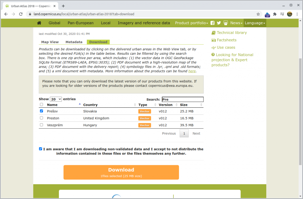
- Local→ Urban Atlas → Urban Atlas 2018: Prešov
- Detailed description of the dataset is available here:
https://land.copernicus.eu/user-corner/technical-library/urban_atlas_2012_2018_mapping_guide_v6-1.pdf
Setup of the environment
Installation of dependencies
- sudo apt install gdal-bin libeccodes0 libgeos-dev python3.8
- gdal-bin – geopandas, rasterio
- libeccodes0 – GRIB support in xarray
- libgeos-dev (maybe libgeos-c1v5 is sufficient) – shapely, cartopy
- Notebooks focused on geopandas, xarray, rasterio were tested with python 3.8
- There are two environments used in this lab (due to compatibility issues with SNAPPY and dask)
- SNAPPY-focused environment (
requirements_OCEA01.txt) - Everything else (
requirements.txt)
- SNAPPY-focused environment (
Applications
- Installation of SNAP:
- Installation of QGIS
- Python 3.X installation
- Follow the installation steps for your specific platform. For instance, nice installation guide is available at https://realpython.com/installing-python/.
Python environment
- Setup of the python environment
- The python and necessary libraries can be installed locally, or the examined jupyter notebooks can be run in cloud-based solutions such as Google colaboratory.
- Environment setup:
- Virtual environments (venv, conda) are recommended for the local installation.
- Virtual environment can be set-up by the following command:
python3 -m virtualenv -p python3 venv
# activation
. venv/bin/activate
- Virtual environment can be set-up by the following command:
- Required non-standard libraries are listed in requirements.txt file
- With pip package installer, all required packages can be installed via:
pip install -r requirements.txt- To resolve Shapely issues:
pip uninstall shapely -ypip install shapely --no-binary shapely
- To resolve Shapely issues:
- Virtual environments (venv, conda) are recommended for the local installation.
- With conda package installer, all required packages can be installed via:
conda env create -f environment.yml- To use files in Google Drive (such as requirements.txt), the Google Drive directories can be mounted in a notebook using google.colab.drive library (see the example notebook). Shell commands can be executed from a jupyter notebook by putting an exclamation point as the first letter of a line (example of shell commands in IPython).
Summary of the lab activities
Lab 1
Loading, visualizing and analysing NetCDF file using xarray – data from Climate Data Store
Demonstration of manipulation with a NetCDF file in xarray library, In this case the coordinates of data points are provided as 2D grids. A data point is provided for each point of the grid. The activity also includes a demonstration of the Climate Data Store provided by Copernicus Climate Change Service (C3S).
Loading, visualizing and analysing NetCDF file using xarray – data from Climate Data Store → Single NetCDF File
- NetCDF – C3S Fire Warning Indicator – single file.ipynb
Loading, visualizing and analysing multiple NetCDF files using xarray – data from Climate Data Store
Demonstration of manipulation with a NetCDF file in xarray library, In this case the coordinates of data points are provided as 2D grids. A data point is provided for each point of the grid. The activity also includes a demonstration of the Climate Data Store provided by Copernicus Climate Change Service (C3S). The activity extends the previous activity by concatenation of NetCDF files and demonstration of vectorized application of a fitting procedure.
Loading, visualizing and analysing NetCDF file using xarray – data from Climate Data Store → Multiple NetCDF Files
- NetCDF – C3S Fire Warning Indicator – multiple files.ipynb
Loading and visualization of NetCDF data from Sentinel-3 (OLCI User products) in xarray
Demonstration of manipulation with a NetCDF file in xarray library, In this case the coordinates of data points are provided as 2D tie points that are not arranged into a grid of points. The activity also includes a demonstration of Copernicus Open Access Hub . The activity extends the previous activity by concatenation of NetCDF files and demonstration of vectorized application of a fitting procedure.
Loading and visualization of NetCDF data from Sentinel-3 (OLCI User products) in xarray
- NetCDF from Sentinel 3 OLCI.ipynb
Loading and visualization of GRIB files in xarray package
The aim of the activity is to demonstrate capability of xarray to work with GRIB files downloaded from the Climate Data Store of C3S. This is demonstrated for a single file and for multi-file dataset. Three methods of reading multi-file datasets are presented.
Loading and visualization of GRIB files in xarray package
- GRIB – C3S Essential climate variables.ipynb
Downloading of Sentinel-2 cloudless data via Web Map Service protocol
A brief demonstration of WMS protocol and Sentinel-2 cloudless dataset provided by EOX. Two approaches are presented, one uses Python and another realizes WMS without any abstraction using wget utility in a short bash script.
Downloading of Sentinel-2 cloudless data via Web Map Service protocol
- WMS s2cloudless.ipynb
Normalized Satellite Indexes in Google Earth Engine
The activity demonstrates Copernicus data access in Google Earth Engine (GEE). It also includes demonstration of the Google Earth Engine API and principle of its operation. The activity shows a different paradigm than the previous lab activities. The task is to calculate NDVI and NDWI indexes using the GEE API.
Normalized Satellite Indexes in Google Earth Engine
- ndvi_ndwi_google_earth_engine.js
- Copy the source code into your’s GEE enviroment
Lab 2
Ship detection in Sentinel-1 data – tutorial OCEA01 by RUS Copernicus
The goal of the activity is to introduce students into Research and User Support (RUS) Copernicus and library of tutorials provided by the portal. In this activity student should gain experience with ESA SNAP application.
Ship detection in Sentinel-1 data – tutorial OCEA01 by RUS Copernicus
Ship detection in Sentinel-1 data using SNAPPY – inspired by tutorial OCEA01 by RUS Copernicus
The activity is a reproduction of previous tutorial, but it realized using SNAPPY package provided by SNAP. The images are handled using numpy library. Visualization is realized using matplotlib and cartopy libraries. The activities include application of GPT operators form python, acquisition of vector data in an instance of SNAP’s product object, dealing with interoperability between SNAPPY and Cartopy, and data visualization in matplotlib and cartopy including reprojections.
Ship detection in Sentinel-1 data using SNAPPY – inspired by tutorial OCEA01 by RUS Copernicus
- OCEA01.ipynb
Lab 3
Per-pixel classification of Sentinel-2 data (inspired by tutorial LAND01 by RUS)
Extensive activity that leads from construction of a dataset of labeled data to application of a trained classifier to unlabeled data of choice. A classifier is trained on an image of Prešov, and a trained model is applied to an image of Košice. The data labels are provided through Urban Atlas 2018, which at the time of preparing this tutorial included data for Prešov, but it did not include data for Košice.
Per-pixel classification of Sentinel-2 data (inspired by tutorial LAND01 by RUS)
- Preparation of the labeled data (products capturing Prešov)
- Per-pixel classification – 1. preparation of datasets – PART1.ipynb
- Per-pixel classification – 1. preparation of datasets – PART2.ipynb
- Per-pixel classification – 1. preparation of datasets – PART3.ipynb
- Training of a random forest classifier on the labeled data
- Per-pixel classification – 2. training.ipynb
- Application of a trained classifier to unlabeled data (products capturing Košice)
- Per-pixel classification – 3. application.ipynb
Preview of Sentinel-2 cloud mask using Geopandas
Supplementary activity to the previous activity focused on visualization of cloud masks and demonstration of cloud types stored in GML files alongside the mask shapes. This activity should be helpful in understanding the extensive product reading procedure used in the previous activity. The activity should be done alongside the previous activity, if explanation of the procedure requires more experimentation.
Preview of Sentinel-2 cloud mask using Geopandas
- Per-pixel classification – misc – cloud masks.ipynb
Other Examples
- Read shapefile in Geopandas.ipynb
- Fiona example.ipynb
More detailed description of lab activities
- Ship detection in Sentinel-1 data – tutorial OCEA01 by RUS Copernicus
- Ship detection in Sentinel-1 data using SNAPPY – inspired by tutorial OCEA01 by RUS Copernicus
- Per-pixel classification of Sentinel-2 data (inspired by tutorial LAND01 by RUS)
- Loading, visualizing and analysing NetCDF file using xarray – data from Climate Data Store
- Loading and visualization of NetCDF data from Sentinel-3 (OLCI User products) in xarray
- Loading and visualization of GRIB files in xarray package
- Downloading of Sentinel-2 cloudless data via Web Map Service protocol
- Normalized Satellite Indexes in Google Earth Engine
Ship detection in Sentinel-1 data – tutorial OCEA01 by RUS Copernicus
The goal of the activity is to introduce students to Research and User Support (RUS) Copernicus and the library of tutorials provided by the portal. In this activity, a student should gain experience with the ESA SNAP application.
The activity is based on tutorial OCEA01 by Copernicus Research and User Support (RUS)
General steps of the activity
- Manual download of the products from Open Hub
- Loading of the data in SNAP GUI
- Analysis of the data using the GUI
- Visualization of data in QGIS
- Visualization of the data in Google Earth
Detailed steps of the activity in SNAP
- Input file
S1A_IW_GRDH_1SDV_20191217T165819_20191217T165844_030391_037A3A_08F2.zip
- Subset: click on different widget (Product Explorer), Subset
- Orbit file
- Radar → Apply Orbit file
- Vector mask
- Vector → Import → ESRI Shapefile
- Ship detection in python https://eodag.readthedocs.io/en/latest/tutorials/tuto_ship_detection.html
https://github.com/CS-SI/eodag/tree/master/examples/auxdata/ Auxiliary files, Gulf_of_Trieste_seamask_UTM33.shp
- Ship detection in python https://eodag.readthedocs.io/en/latest/tutorials/tuto_ship_detection.html
- Vector → Import → ESRI Shapefile
- Ship detection
- Radar → SAR Applications → Ocean Applications → Ocean Object Detection
- Land-Sea-Mask
- Calibration
- The radiometric correction is necessary for the pixel values to truly represent the radar backscatter of the reflecting surface
- Adaptive Thresholding
- Object Discrimination
- Radar → SAR Applications → Ocean Applications → Ocean Object Detection
- Export the results to Shapefile
- Vector Data, ShipDetections, Geometry as a Shapefile
- Error in SNAP
Processing/subset_S1A_IW_GRDH_1SDV_20161009T165807_Orb_Cal_THR_SHP.data/vector_data/ShipDetections.csv- data is still not projected to a known projection such as WGS84
- However, a temporary file with coordinates is located here
~/.snap/var/log/subset_S1A_IW_GRDH_1SDV_20161009T165807_4550_Orb_Cal_THR_object_detection_report.xmlxmllint --xpath "//target/@*[name()='Detected_lat' or name()='Detected_lon' or name()='Detected_length']" "$f" | sed -r 's/ ?Detected_lat="([^"]+)" Detected_lon="([^"]+)" Detected_length="([^"]+)"/\1;\2;\3\n/g' > "$outdir/obeject_detection_report_lat_lon_length.csv"- Consider extracting other fields
- Load the Shapefile mask into QGIS via browser
- Add Delimited Text Layer, different UI in QGIS 3 to QGIS 2
- X field longitude (filed_2), Y field latitude (filed_1)
- Find Coordinate Reference System WGS84 with ID: EPSG: 4326
- Layers: Save as (shp) / Export>Export features as
- Background map
- via MapTiler (requires registration and API key)
- Via QuickMapServices, search QMS “world”
- ESRI Satellite, EOX::Maps Sentinel-2 cloudless
- ESRI World topo, Waze World – notice deformations
- Maps with red dot does not work, yellow nothing visible
- Layers: detections layer > Labels > Single labels (QGIS 3) / Show labels for this layer (QGIS 2)
- Save Feature As > Format: KML
- Vector Data, ShipDetections, Geometry as a Shapefile
Ship detection in Sentinel-1 data using SNAPPY – inspired by tutorial OCEA01 by RUS Copernicus
The activity is a reproduction of the previous tutorial, but it realized using the SNAPPY package provided by SNAP. The images are handled using NumPy library. Visualization is realized using Matplotlib and Cartopy libraries. The activities include the application of GPT operators form python, acquisition of vector data in an instance of SNAP’s product object, dealing with interoperability between SNAPPY and Cartopy, and data visualization in Matplotlib and Cartopy including reprojections.
Before running this notebook:
- Install SNAP
SNAP_INSTALLvariable is used as a placeholder representing installation directory
- Symlink
gptutility into working directory of this notebookln -s $SNAP_INSTALL/bin/gpt
- Run
snappy-confutility- At this time (january 2021) SNAPPY does not work with Python 3.8, Python 3.6.9 works.
"$SNAP_INSTALL/bin/snappy-conf" "$(realpath venv_snappy/bin/python)" "$(realpath .)"- If snap GUI is not opened, the program is stuck after directory creation (seems to be IPC error). The process can be interrupted via Ctrl+C.
Guides to setup Snappy:
- Marco Peters. SNAP Wiki: Configure Python to use the SNAP-Python (snappy) interface
- Roman Shevchuk et al. SNAP Wiki: How to use the SNAP API from Python
Steps
- Reading the product file via SNAPPY API
- Visualization of bands using matplotlib
- Application of GPT operators
- Subset,
- Apply Orbit File,
- Application of land-sea mask,
- Calibration,
- Object detection
- Adaptive thresholding,
- Object discrimination
- Forced loading of raster data
- Retrieval of a vector data group from a product
- Datatype casting operation via jpy
- Acquisition of a list of GeoTools’s SimpleFeature objects.
- Reading of SimpleFeature object attributes
- Creating Geopandas dataframe (GeoDataFrame)
- Recalculation of pixel grid points form centers to edges
- Visualization using cartopy including reprojection into EuroPP CRS.
- Preview of an alternative approach using GPT utility
Tasks
TASK #1: Complete implementation of the visualization function output_view
- Get a reference to a band object from a product and assign it to variable
band. Locate appropriate function in API reference and assing the result to variableband. - Read band data into a numpy array. Hint: Use a variant of
readPixels()method which does not have a progress monitor parameter. - See:
TASK #2: Apply Land-Sea mask to the product from previous operation (orbit_applied_product)*
- First, use
Import-Vectoroperator to import a vector fileGulf_of_Trieste_seamask_UTM33.shp - Second, use
Land-Sea-Maskoperator to apply the mask to the product.
TASK #3: Create a GeoDataFrame of detected ships
- Use SNAP’s Product Data Model to access the features collection in a
VectorDataNode(ship_detections_vector) and store each as a point in the table’s geometry column - The data frame should have the following columns:
geometry,det_w,det_hdet_w– a simple feature’s attribute"Detected_width"det_h– a simple feature’s attribute"Detected_height"geometry– an instance ofshapely.geometry.Pointwhich coordinates are determined by attributes'Detected_lon'and'Detected_lat'
- Store results in a
geopandas.GeoDataFramereferenced by a variableship_detections_gdf - See:
Per-pixel classification of Sentinel-2 data (inspired by tutorial LAND01 by RUS)
Extensive activity that leads from construction of a dataset of labeled data to application of a trained classifier to unlabeled data of choice. A classifier is trained on an image of Prešov, and a trained model is applied to an image of Košice. The data labels are provided through Urban Atlas 2018, which at the time of preparing this tutorial included data for Prešov, but it did not include data for Košice.
Preparation of the labeled data (products capturing Prešov)
Steps
- Manual download of the data from Copernicus Land Monitoring Service (Urban Atlas 2018)
- Loading Land Monitoring Service Data in Geopackage format
- Comparison of map projections available in Cartopy
- Inverse transformation of coordinates using Proj (Pyproj) library
- Downloading administrative region shapefiles from Natural Earth Data using cartopy
- Visualization of GeoDataFrame alongside Shapely polygon data
- Download of specific product files (quicklook images) using OData protocol directly (without any abstraction)
- Downloading the data from Copernicus Open Hub – OpenSearchAPI, OData using sentinelsat package
- Extracting the downloaded product data
- Navigating Sentinel-2 product data
- Saving GeoDataFrame as GeoJSON
- Reading clouds mask in GML format using Geopandas
- Preparation of cloud and footprint raster masks
- Windowed reading raster band data using rasterio
- Masking of band image data
- Reprojection in rasterio
- Visualization of raster data alongside vector data
- Saving band images in npz
- Saving band images in NetCDF
Tasks
TASK #1: Use appopriate Geopandas function to load GeoPackage file into a GeoDataFrame
TASK #2: Use appopriate parameters of GeoDataFrame.plot() function to categorize data by column class_2018
TASK #3: Filter-out LMS data with specific codes
- Create a view of the GeoDataFrame
lms_po_all_gdfwhich contains only entries with the following codes (usecode_2018column):31000– Forests11100– Continuous urban fabric (S.L. : > 80%11210– Discontinuous dense urban fabric (S.L. : 50% – 80%)11220– Discontinuous medium density urban fabric (S.L. : 30% – 50%)21000– Arable land (annual crops)
TASK #4: Transform LMS data bounds into longitude/latitude
- The recommended approach is to transform the CRS into
EPSG:4326(see https://epsg.io/4326) - Make sure to provide longitude and latitude in degrees
- See:
- https://pyproj4.github.io/pyproj/stable/advanced_examples.html
- https://pyproj4.github.io/pyproj/stable/api/transformer.html#pyproj.transformer.Transformer.transform
- https://gis.stackexchange.com/questions/78838/converting-projected-coordinates-to-lat-lon-using-python
- https://shapely.readthedocs.io/en/stable/manual.html#other-transformations
- https://pyproj4.github.io/pyproj/dev/api/proj.html
- Usage of
always_xy=Trueis highly recommended
TASK #5: Construct bounding box polygon
- Use appropriate Shapely geometry function
TASK #6: Use appropriate SentinelAPI functions to download all products in a list
- Product identifiers are in the column
uuidofproducts_to_download_df - Save product files into directory in variable
product_download_dir - See: https://sentinelsat.readthedocs.io/en/stable/api.html
TASK #7: Rasterize the Clouds/Clear-sky mask
- Clouds/Clear-sky mask is loaded completly
- No cropping is applied.
- The mask is inverted
- Thus, the returned window should be None and the returned value is ignored.
TASK #8: Load the first (and only) band from the file
- The data should be loaded using a window only containg the data of the interest
- Load the data into a masked array
TASK #9: Apply the reprojection to the band data
- Use the windowed transform of the data of interest
- Provide the appropriate CRSs
- Use the
dst_crsas the destination transform
BONUS TASK: Save the output data as NetCDF
- Save the produced dataset in NetCDF files, one file per product
- Provide proper coordinates in the CRS of the the band images
Training of a random forest classifier on the labeled data
Steps
- Loading npz files
- Flattening of band image data
- Preparation of training and testing sets
- Training of a random forest classifier (using the first downloaded product)
- Cross-validation
- Visualization of the classification results
- Application of the classifier to other product
Tasks
TASK #1: Load GeoJSON file 'products_of_interest_gdf.json' into a GeoDataFrame
- Use an appropriate Geopandas function
- Don’t forget to set an appropriate column as an index
- See:
TASK #2: Load CSV file 'lms_class_names.csv' into DataFrame
- Use an appropriate Pandas function
- See: https://pandas.pydata.org/pandas-docs/stable/user_guide/10min.html#getting-data-in-out
TASK #3: Create an appropriate supervised classifier available in Scikit-learn API
- Recomennded classifier is RandomForestClassifier due to its fast training time.
- It is recommented to set verbosity level to 1.
- If algorithm supports parallel processing, configure
n_jobsparameter. - It is recommended to set
class_weighttobalancedto accomodate for uneven class fequencies in the training data. - In case of decision tree-based methods, set
min_samples_splitormin_samples_leafto greater than default values, or the tree depth (max_depthparameter). - See:
TASK #4: Run classification for all products in sorted_products_of_interest_df
- You can base the entire source code for this task on the previous examples.
- Observe the classification results.
- Think about possible explanation for varying accuracy between the products.
TASK #5: Duplicate this notebook and modify this condition to include more products
- After the activities in this notebook are complete, continue with this step.
- Perform the modification and run the updated notebook. Then compare results between the two models.
- More sophisiticated approach would use several images in percisely selected temporal windows, each would serve as an input to the classifier, and not just as another datapoint of the training set.
Application of a trained classifier to unlabeled data (products capturing Košice)
Steps
- Geolocation of “Kosice, Slovakia”
- Downloading the data from Copernicus Open Hub – OpenSearchAPI, OData
- Extracting the downloaded product data
- Reading clouds mask in GML format using Geopandas
- Windowed reading raster band data using rasterio
- Masking of band image data
- Reprojection in rasterio
- Loading trained model
- Flattening of band image data
- Application of a trained classifier
- Visualization of the classification results
Tasks
TASK #1: Use appopriate Geopy function to retreive longitude and latitude of Kosice, Slovakia, then construct a WKT string denoting a point.
- Geopy documantation: https://geopy.readthedocs.io/en/stable/#specifying-parameters-once
- WKT: https://en.wikipedia.org/wiki/Well-known_text_representation_of_geometry
- Store the resulting WKT point in the variable
ke_point_wkt
TASK #2: Use appropriate SentinelAPI functions to search for products matching the criteria
- Search for product Sentinel-2 MSI Level 1C products (
'S2MSI1C') that intersect Kosice (ke_point_wkt), and the sensing time (date) of the product is 20 days before or after May 1, 2020 (product_mean_datetime). - See: https://sentinelsat.readthedocs.io/en/stable/api.html
TASK #3: Load the existing classifier created in the previous notebook
- Use
jobliblibrary - See: https://scikit-learn.org/stable/modules/model_persistence.html
Preview of Sentinel-2 cloud mask using Geopandas
Supplementary activity to the previous activity focused on visualization of cloud masks and demonstration of cloud types stored in GML files alongside the mask shapes. This activity should be helpful in understanding the extensive product reading procedure used in the previous activity. The activity should be done alongside the previous activity, if explanation of the procedure requires more experimentation.
Steps
- Navigating Sentinel-2 product data
- Reading clouds mask in GML format using Geopandas
- Visualization of cloud masks
Loading, visualizing and analysing NetCDF file using xarray – data from Climate Data Store
Single NetCDF File
Demonstration of manipulation with a NetCDF file in xarray library, In this case the coordinates of data points are provided as 2D grids. A data point is provided for each point of the grid. The activity also includes a demonstration of the Climate Data Store provided by Copernicus Climate Change Service (C3S).
Steps
- Manual download of the data from Copernicus Climate Change Service (data from fire danger indicator models)
- Overview of the data in Panoply
- Usage of latitude and longitude grids provided in the data
- Visualization of data
- Analysis of latitude and temporal dependence of variables (fire danger indicator)
- Binning values by latitude, and calculation of a mean fire danger indicator value per latitude bin
- Visualization of the data in line plots
Tasks
- TASK #1: Plot mean FWI value (
fwi-mean-jjas) infwi_2010_dsinto an individual plot for each time step ('time')- This is a single function call
- There should be a map of Europe plotted for each time step
- At this time do not be concerned with a proper projection of the data
- See: http://xarray.pydata.org/en/stable/plotting.html
- TASK #2: Plot mean FWI value (
fwi-mean-jjas) in the first data array offwi_2010_dsbut specifyx='lon'andy='lat'- This is a single function call
- Use parameters:
x='lon'andy='lat' - See:
- TASK #3: Plot mean FWI value (
fwi-mean-jjas) in datasetfwi_2010_dsinto an individual plot for each time step ('time') and specifyx='lon'andy='lat'- This is a single function call
- There should be a map of Europe plotted for each time step
- Use parameters:
x='lon'andy='lat' - See:
- TASK #4: Bin dataset
fwi_2010_t0alongside the latitude (lat) dimension into 5 bins - TASK #5: For each group of
fwi_2010_t0_groupby_lat_bins, reduce FWI values (fwi-mean-jjas) into a single mean value over all dimensions of a dataset associated with the group. - TASK #6: Bin dataset
fwi_2010_dsalongside the latitude (lat) dimension into 5 bins- Replicate steps done for
fwi_2010_t0 - See: http://xarray.pydata.org/en/stable/groupby.html#binning
- Replicate steps done for
- TASK #7: For each group of
fwi_2010_groupby_lat_bins, reduce FWI values (fwi-mean-jjas) into a single mean value over all dimensions of a dataset associated with the group.- Replicate steps done for
fwi_2010_t0 - See:
- Replicate steps done for
Multiple NetCDF Files
Demonstration of manipulation with a NetCDF file in xarray library, In this case the coordinates of data points are provided as 2D grids. A data point is provided for each point of the grid. The activity also includes a demonstration of the Climate Data Store provided by Copernicus Climate Change Service (C3S). The activity extends the previous activity by concatenation of NetCDF files and demonstration of vectorized application of a fitting procedure.
Steps
- Concatenation of xarray datasets
- Visualization of the data
- Analysis of latitude and temporal dependence of variables (fire danger indicator)
- Fitting fire danger indicator value in time to polynomials for a single latitude bin
- Analysis of the data for all latitude bins along the time dimension
- Vectorized application of the fitting procedure
Tasks
- TASK #1: Concatenate datasets in the list
fwi_ds_listalongside the time dimension - TASK #2: Concatenate datasets in the list
fwi_ds_listalongside the time dimension, but include only datasets with 5 time steps. Then sort dataset arrays by time in ascending order.- Filter-out datasets which do not have 5 steps in the time dimension
- Concatenate datasets which passed the filter
- Sort arrays of the new dataset alongside the time dimension
- See:
- TASK #3: Bin dataset
fwi_dsalongside the latitude (lat) dimension into 10 bins - TASK #3: Fit first-order polynomial function parameters to FWI data as a function of time in array referenced by variable
mean_fwi_xarr_lat_0 - TASK #4: Fit third-order polynomial function parameters to FWI data as a function of time in array referenced by variable
mean_fwi_xarr_lat_0- Polynomial of the first degree (
deg=3) - Add parameter
full=Trueand observe the result - See:
- Polynomial of the first degree (
- TASK #5: Plot mean FWI value (
fwi-mean-jjas) inmean_fwi_xarrinto an individual plot for each latitude bin ('lat_bins')- This is a single function call
- See the plotting example above
- See: http://xarray.pydata.org/en/stable/plotting.html
- TASK #6: Fit first-order and third-order polynomial function parameters to FWI data as a function of time in array referenced by variable
mean_fwi_xarr- Polynomial of the first degree and third degree (
deg=1,deg=3) - Observe the dimensionality of returned datasets
- See:
- Polynomial of the first degree and third degree (
Loading and visualization of NetCDF data from Sentinel-3 (OLCI User products) in xarray
Demonstration of manipulation with a NetCDF file in xarray library, In this case the coordinates of data points are provided as 2D tie points that are not arranged into a grid of points. The activity also includes a demonstration of Copernicus Open Access Hub . The activity extends the previous activity by concatenation of NetCDF files and demonstration of vectorized application of a fitting procedure.
Steps
- Loading multiple NetCDF files in xarray, usage of dask library
- Loaded files include geo coordinates (tie_goeCoordinates),
- Merging of xarray datasets
- Visualization a lat/lon-dependent variable (total ozone)
- Optimization of visualization performance
- Visualization a lat/lon-dependent variable (global vegetation index) using Cartopy
Tasks
- TASK #1: Visualize Global Vegetation Index in dataset referenced by variable
ogvi_ds- Base your code on the examples above.
- Recommended colormap is
"brg"
Loading and visualization of GRIB files in xarray package
The notebook for this activity demonstrates reading GRIB using xarray. This is demonstrated for a single file and for multi-file dataset. Three methods of reading multi-file datasets are presented.
Downloading of Sentinel-2 cloudless data via Web Map Service protocol
A brief demonstration of WMS protocol and Sentinel-2 cloudless dataset provided by EOX. Two approaches are presented, one uses Python and another realizes WMS without any abstraction using wget utility in a short bash script.
Steps
- Access the data using OWSLib package
- Review of WMS metadata
- Download of the data, storing the data in a file, efficient visualization in a Jupyter notebook
- Access the data using a bash script
Tasks
- TASK #1: Specify bounding box parameters to download a map for the whole planet
- You can utlize bound accessible through
wms.contents['s2cloudless_3857'].boundingBox - See https://epsg.io/900913
- You can utlize bound accessible through
- TASK #2: Select 20x20km box around Kosice, Slovakia
- TASK #3: Downloading data via WMTS protocol
- This can be implemented as a bash script outside of this notebook, or it can be implemented in the cell below
- Manually review https://tiles.maps.eox.at/wmts/1.0.0/WMTSCapabilities.xml
- Find layer
s2cloudless-2019 - Find
TileMatrixSetfor this layer - Within this
TileMatrixSetchooseTileMatrixwithIdentifiervalue equal1 - Identify values for
ServiceTypeVersion, the layer’s style, MIME format - Either use resource URL from the
WMTSCapabilities.xmlor do a proper WMTSGetTilerequest${SERVER_URL}?SERVICE=WMTS&REQUEST=GetTile&VERSION=${VERSION}&LAYER=${LAYER}&STYLE=${STYLE}&FORMAT=${FORMAT}&TILEMATRIXSET=${TILEMATRIXSET}&TILEMATRIX=${TILEMATRIX}&TILEROW=${i}&TILECOL=${j}
- Save the output into
ows_data_download/WMTSdirectory - To download an image you can use
wgetutility
- Find layer
Normalized Satellite Indexes in Google Earth Engine
The activity demonstrates Copernicus data access in Google Earth Engine (GEE). It also includes demonstration of the Google Earth Engine API and principle of its operation. The activity shows a different paradigm than the previous lab activities. The task is to calculate NDVI and NDWI indexes using the GEE API.
Tasks
- TASK #1: Provide the equation for NDVI and rename the band to “NDVI”
- TASK #2: Provide the equation for NDVI and rename the band to “NDWI”
Some links
- https://developers.google.com/earth-engine/datasets/catalog/COPERNICUS_S2
- https://developers.google.com/earth-engine/guides/image_overview
- https://developers.google.com/earth-engine/guides/image_math
- https://developers.google.com/earth-engine/apidocs/ee-image-reduceregion
- https://developers.google.com/earth-engine/guides/client_server
- https://developers.google.com/earth-engine/guides/deferred_execution
Incomplete list of recommended reading (and video)
General information
- Introduction to Remote Sensing
- Lessons: https://www.learn-eo.org/
- https://earth.esa.int/web/guest/eo-education-and-training
Slides
- Jochen Albrecht. 201 Lectures (Introduction to Mapping Sciences). Hunter College, City University of New York http://www.geo.hunter.cuny.edu/~jochen/gtech201/lectures/
- For instance, extensive material on projections: How to choose a projection
- Course/summer school: Satellite Image Analysis | Special Interest Group at UW eScience Institute (https://uwescience.github.io/sat-image-analysis/)
- Summary of resources: Satellite Image Analysis Reference Guide | Satellite Image Analysis
- Slides from workshops focused on Sentinel data processing
http://ftp.itc.nl/pub/Dragon4_Lecture_2019
Courses
- ESA MOOCs (Massive Open Online Courses)
- https://earth.esa.int/web/guest/eo-education-and-training/moocs
- Echoes from space: Introduction to Radar Remote Sensing
https://eo-college.org/courses/echoes-in-space/, EO College (YouTube) - Earth Observation from Space: the Optical View
https://www.futurelearn.com/courses/optical-earth-observation - Monitoring Climate from Space
https://www.futurelearn.com/courses/climate-from-space
- Earth observation summer school
- Books:
- Surekha Borra, Rohit Thanki, Nilanjan Dey. Satellite Image Analysis: Clustering and Classification
- Thomas M. Lillesand Ralph W Kiefer Jonathan Chipman. Remote Sensing and Image Interpretation
- Joel Lawhead. Learning Geospatial Analysis with Python: Understand GIS fundamentals and perform remote sensing data analysis using Python 3.7 (2019)
- Paul Crickard, Eric van Rees, Silas Toms. Mastering Geospatial Analysis with Python. Packt Publishing. (2018))
- Thomas M. Lillesand, Ralph W Kiefer, Jonathan Chipman. Remote Sensing and Image Interpretation (2015, Wiley)
- David DiBiase et al. The Nature of Geographic Information (An Open Geospatial Textbook). PennState College of Earth and Mineral Sciences. Available at: https://www.e-education.psu.edu/natureofgeoinfo/
Courses (in a book form)
- United States Naval Academy, Professor Peter L. Guth. MICRODEM Help Home Page
- Documentation which includes resources in a book-like/course-like form
- Example: Normalized Satellite Indexes
- Homepage: https://www.usna.edu/Users/oceano/pguth/website/plghome.htm
- Courses/Tutorials
- Copernicus Research and User Support (https://rus-copernicus.eu/)
- Virtual machines
- Youtube channel
- Mainly SNAP-based tutorials
- Tutorials in PDF: https://rus-copernicus.eu/portal/the-rus-library/train-with-rus/
- Course Automating GIS-processes 2019 by University of Helsinki, Finland.
(2018 version) - Course Geo-Python 2020 by University of Helsinki, Finland.
- Free Earth Data Science Courses & Textbooks
- Many course materials
- For instance: Scientist’s Guide to Plotting Data in Python Textbook Earth Lab CU Boulder , Earth Data Analytics Online
- Course Introduction to Geospatial Concepts by Data Carpentry
- Course Geospatial Data Visualization (Cartopy, Geopandas) developed to support Geohackweek workshop
- Prof P. Lewis. UCL. GeogG122: Scientific Computing
- Extensive material
- Some examples:
- 10. Pull MODIS data via FTP – Read an HDF file (e.g. MODIS data products)
- 11. Read and use some different file formats
- 12. Apply a vector mask to a Raster image
- Introduction to Geospatial Raster and Vector Data with Python by carpentries-incubator.
- WUR Geoscripting course. Wageningen
- Raster and vector data processing in R and Python
- For example: https://geoscripting-wur.github.io/PythonVector/
- Course: Getting your hands-on Climate data – Working with Copernicus Climate Data Store (CDS)
- EUMETSAT YouTube Channel (For instance Visualising data in NetCDF format)
- NASA Earthdata
Tutorials, Jupyter notebooks
- GEARS (https://www.gears-lab.com/)
- Google Earth Engine Tutorials and others
- Youtube channel: https://www.youtube.com/channel/UCPZMj2ykE9pgJGV1r0kXQMg
- EarthPy – a collection of IPython notebooks with examples of Earth Science related Python code. http://earthpy.org/
Supporting python package: EarthPy: A Python Package for Earth Data — EarthPy 0.9.2 documentation - Google Earth Engine’s tutorial resources
- Planet Lab’s jupyter notebooks
- Extensive series of Geospatial data analysis tutorials and inspirational body of work by Patrick Gray
- Personal website: http://patrickgray.me/
- Open Source Geoprocessing Tutorial (https://github.com/patrickcgray/open-geo-tutorial)
- Introduction [HTML]
- The GDAL datatypes and objects [HTML]
- Your first vegetation index [HTML]
- Visualizing data [HTML]
- Vector data – the OGR library [HTML]
- Land cover classification [HTML]
- Deep Learning for land cover classification [HTML] built to run in Google Colab.
- Earth Engine for Oceanographic Time Series Analysis [HTML]
- A Stock Scientific Computing / Deep Learning Environment for Analysis of Remote Sensing Data
https://github.com/patrickcgray/sci_compute_env - patrickcgray / notebooks (fork of planetlab’s tutorials)
- Support materials for FOSS4G-CEE-2013 Python-GIS workshop
https://github.com/GISMentors/geopython-zacatecnik/tree/english - Specific one-off tutorials
- Sentinel-2 image clustering in python | by Wathela Hamed
- Mask R-CNN for Ship Detection & Segmentation
- Ryan Abernathey. Maps in Scientific Python. (Cartopy tutorial)
https://rabernat.github.io/research_computing_2018/maps-with-cartopy.html - Sentinel-1 InSAR Processing using the Sentinel-1 Toolbox https://asf.alaska.edu/wp-content/uploads/2019/05/generate_insar_with_s1tbx_v5.4.pdf
- M. Fraiser. Overview of Coordinate Reference Systems (CRS) in R. https://www.nceas.ucsb.edu/sites/default/files/2020-04/OverviewCoordinateReferenceSystems.pdf (like a cheatsheet)
- Joshua Hrisko. Geographic Visualizations in Python with Cartopy on https://makersportal.com/
Lists
- https://github.com/robmarkcole/satellite-image-deep-learning
- Extensive list of references and analyses, nice examples
- https://github.com/sacridini/Awesome-Geospatial
- List of geospatial analysis tools
- Essential geospatial Python libraries | by Christoph Rieke | Medium
- Shortlist with explanation
- ESA’s Earth online portal
- https://earth.esa.int/eogateway/
- Data, tools, Events, Missions, Instruments, Activities, Campaigns, Documents
- Specific tools/libraries
- SNAP
- SNAP HELP
- SNAP Wiki https://senbox.atlassian.net/wiki/spaces/SNAP/overview?homepageId=1605639
- Orfeo ToolBox – potentially useful library (https://www.orfeo-toolbox.org/)
- Articles:
- Sayon Kumar Saha. Satellite Imagery Analysis: Kerala Flood
- Geoparsing module created in this work (reading Sentinel-2 data): https://github.com/sayonkumarsaha/satellite-index-earth-observation-experiement/tree/master/geoparsing
- Improving Cloud Detection with Machine Learning | by Anze Zupanc | Sentinel Hub Blog
Datasets
- https://asf.alaska.edu/ – Distributed Data Archive Center
- Database of SAR data including Sentinel-1
- Earth Observation data on Amazon AWS
- Socioeconomic Data and Applications Center | SEDAC
Other
- OGC Abstract Specification Topic 2: Referencing by coordinates
- Annex B – Spatial referencing by coordinates – Geodetic concepts (informative)